How to create a drop-down list in Excel: complete step-by-step guide

A drop-down list in Excel allows users to choose a value from predefined options instead of typing manually. This helps prevent errors, keeps data consistent, and makes spreadsheets easier to use, especially when shared with others.

Microsoft provides a built-in feature called Data Validation that lets you create a drop-down list in just a few clicks. No formulas or coding are required.

This guide explains the full setup process step by step, including what appears on screen.

Step 1: Prepare the list items in Excel

Before creating a drop-down list, you need the values that will appear inside it.

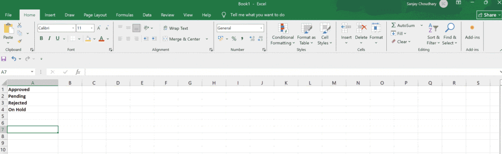
1. Open Excel and create a new worksheet.
2. In a single column, type the list values.
   • Example:
     • Cell A1: Pending
     • Cell A2: Approved
     • Cell A3: Rejected

These values will act as the source for your drop-down list.

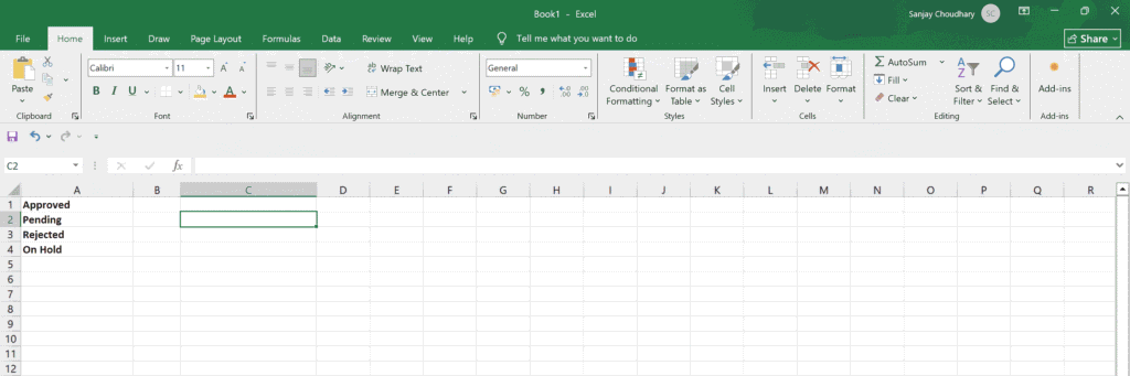
Step 2: Select the cell where the drop-down list will appear

1. Click on the cell where you want the drop-down list.
   • Example: Cell C2

This is the cell users will click to select values.

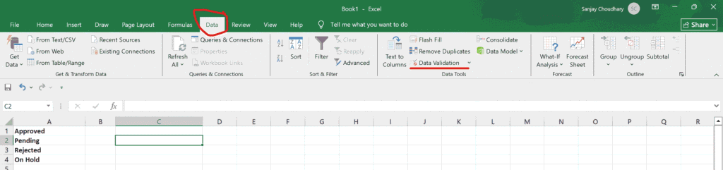
Step 3: Open the Data Validation settings

1. Go to the top Excel ribbon.
2. Click the Data tab.
3. In the Data Tools group, click Data Validation.
4. From the dropdown, select Data Validation again.

A settings window will open.

Screenshot tip:
Take a screenshot showing:

• The Data tab highlighted
• The Data Validation button visible

Step 4: Configure the drop-down list settings

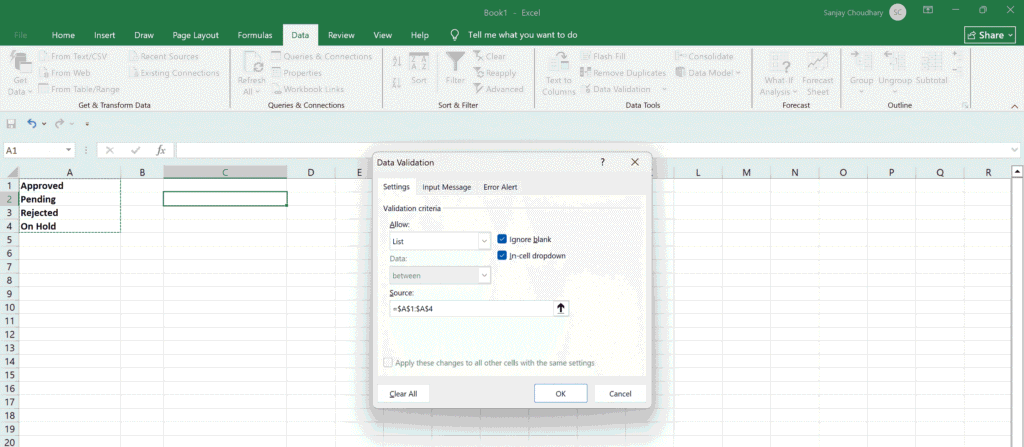
In the Data Validation window:

1. Under the Settings tab:
   • Click the Allow dropdown
   • Select List
2. Click inside the Source box.
3. Select the cells that contain your list values.
   • Example: Select A1 to A3
4. Make sure In-cell dropdown is checked.
5. Click OK.

The drop-down list is now created.

• Allow set to List
• Source showing the selected range

Step 5: Test the drop-down list

1. Click the cell where the drop-down list was created.
2. Click the small arrow that appears.
3. Select one of the values.

Excel will only allow values from the list.

Step 6: Add an input message (optional but useful)

Input messages guide users when they click the cell.

1. Open Data Validation again.
2. Go to the Input Message tab.
3. Check Show input message when cell is selected.
4. Enter:
   • Title: Select status
   • Message: Choose one option from the list
5. Click OK.

Screenshot tip:
Capture the Input Message tab filled in.

Step 7: Set an error alert for invalid entries

This prevents users from typing values outside the drop-down list.

1. Open Data Validation.
2. Go to the Error Alert tab.
3. Check Show error alert after invalid data is entered.
4. Choose:
   • Style: Stop
   • Title: Invalid entry
   • Message: Please select a value from the drop-down list
5. Click OK.

Now Excel will block incorrect entries.

Screenshot tip:
Take a screenshot of the Error Alert tab and another of the error message popup.

Step 8: Create a dynamic drop-down list (advanced)

If you want the drop-down list to update automatically when new values are added:

1. Select your list values.
2. Go to Formulas → Define Name.
3. Give it a name like StatusList.
4. Use that name in the Data Validation Source field instead of cell references.

This method is ideal for large or frequently updated lists.

Why using a drop-down list improves Excel accuracy

A drop-down list reduces typing errors, enforces consistency, and makes spreadsheets easier to analyze. It is especially useful in finance, HR, reporting, inventory tracking, and dashboards.

Because all entries come from a fixed list, formulas, charts, and pivot tables work more reliably.

Read Also: Itaú Asset Management recommends 1% to 3% Bitcoin allocation for 2026